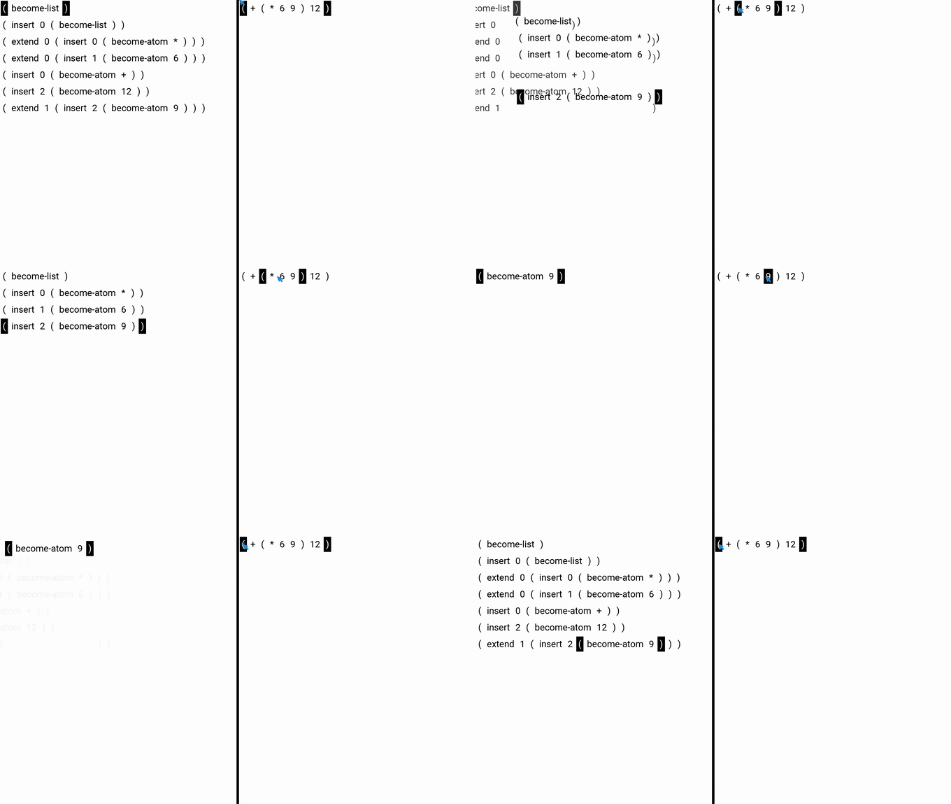
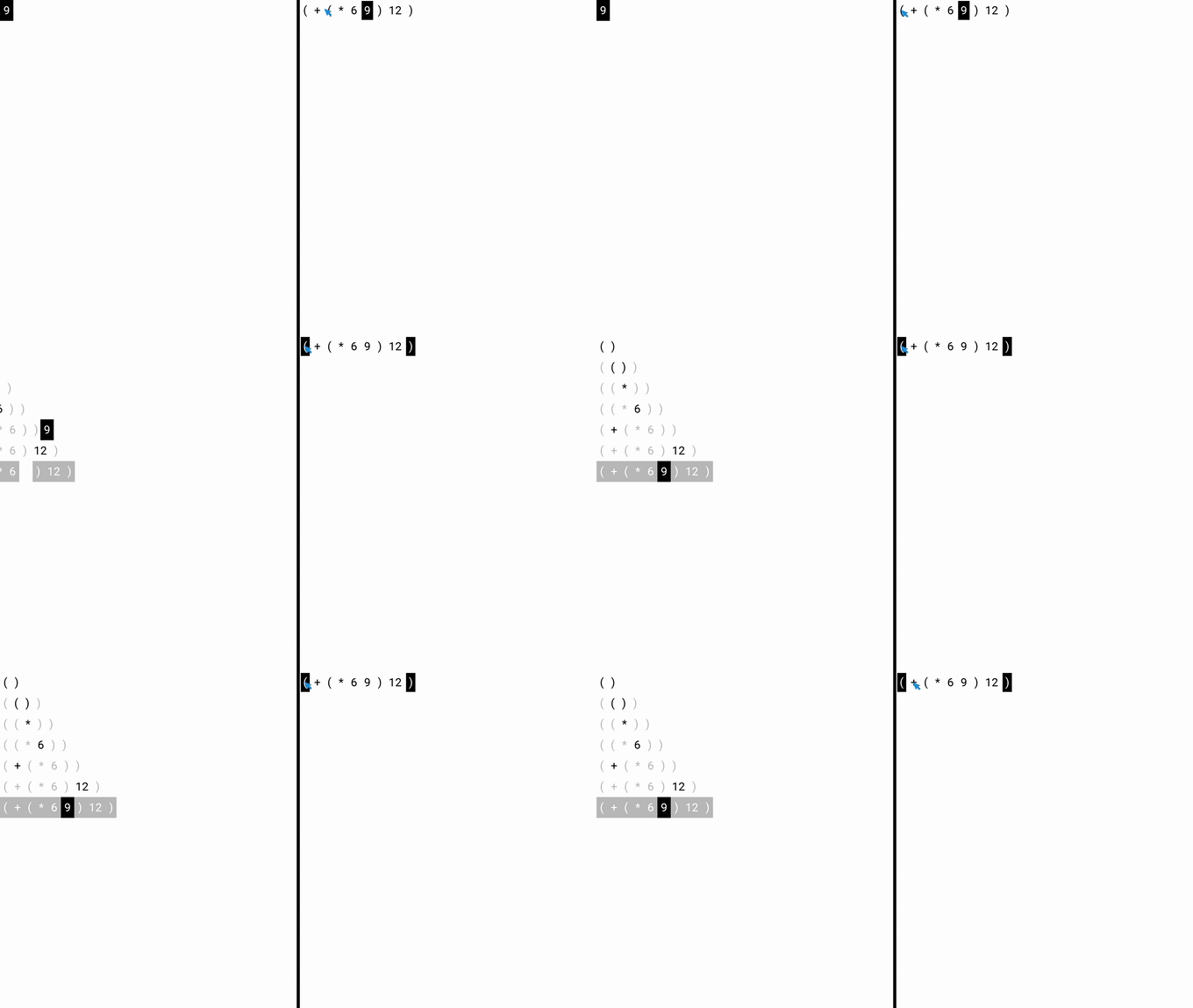
Animating history: Implementation
Oct 16, 2018 — Tags: The editor
In the previous article we have seen how we can show animations in the history pane of the editor to subtly illustrate how the construction of different levels of our program relate to each other. Here we provide some notes on these animations are implemented.
What are history-animations?
History-animations build on the following feature (one that was already existing): whenever we select an s-expression in our “tree” (the structural view on the right hand side of the window) we show the history of that particular s-expression in the panel on the left. That is, whenever we change the cursor in the tree, we switch what is shown in the history.
The animation under discussion: any part of history that shows up both before and after this switch will “float” from its pre-switch position to its post-switch position in a number of steps. The idea is to make it visually more clear that there is a relationship between the histories at different levels of the tree.
More details and examples can be found in a separate article. In the present article we’ll zoom in on the implementation.
The current version of the editor supports 2 versions of rendering histories: one in which the histories are rendered as s-expressions themselves, as presented in the paper the paper “Clef Design”; one in which the effects of each note are shown in the context of the structure on which it is played (i.e.: more like a traditional rendering of a diff). Animations of transitions are implemented for both of these; where the implementations diverge this will be pointed out in the below.
Identity of notes and textures
The key idea in the animations is to float textures from some pre-switch to a post-switch location. This hinges on the assumption that we have a shared identity for the textures pre- and post-switch. E.g. to float some open-bracket from one location to the next, we need to know which open-bracket we’re talking about (there are many, and they look very similar).
Note that the particular animation under consideration is the following: when swichting which part of our structural view (the “tree”) is selected, update the historical view.
Thus, the assumption of shared identity, in this case, is: there is overlap between the histories of different parts of our tree. For each of the elements (notes) of the history we can establish an identity, and when viewing a different history, we can establish whether any two notes across these two histories are the same one, i.e. share this identity.
The fact that parts of histories are shared across different parts of our structure is detailed in the paper “Clef Design”
In terms of the implementation, the solution is to have some addressing scheme for the textures that is global in the sense that it is shared between the pre-and post-switch environments. Using this addressing scheme we can identify textures: same address means same texture.
Such an addressing scheme for textures is obtained in a number of steps.
NoteAddress
The first step is to annotate each note in the “global history” (the history of the whole tree) in such a way that we can uniquely identify each note. Implementation and calling locations
The formalization of the note-address is implemented in the class NoteAddress
The intuition here is: when the whole history is written out as an expression, the address of a particular note is a path trough that expression. An example could be: of the global score, take the 6th item; of that item take the only child, of that item again take the only child. The 2 main possible parts of such paths are: the nth item of a Score, and the only child. The doctests provide further details.
Push global NoteAddress to the tree
In the second step, we construct a tree by playing this global history of notes, annotated with their global address (here and here). We use the regular mechanism of playing a score to get a tree (This one – in fact, it’s not 100% identical for implementation reasons, as documented in the code, but in terms of behavior it is). The only difference is: because the input Notes have now been annotated with a global address, the scores as constructed at each sub-expression in the resulting tree are now consisting of notes which have a global address. This means that when we fetch the “local score” (the score to be rendered) we have information about the global address of each note.
Texture-addresses
Finally, we make sure to keep the annotations around in each step of the conversion to textures, as well as add conversion-specific information when needed. The implementations of this final step are unique for each of the two different styles of rendering.
ELS’18 style rendering
In the case rendering of in the style of the ELS’18 paper, the tree of notes is first converted to an s-expr, and these s-expressions are then converted to the actual textures with locations.
We need step-specific address information for each of these steps. When converting to
an s-expression, we annotate the elements that are specific to the fact that the
note is being rendered as an s-expression (i.e. the fact that the Note’s fields
and its type, when converted to an s-expression, turn into particular
further s-expressions). Let’s consider the case of become-atom as an
example:
when the note (become-atom foo) is represented as an s-expression the whole
s-expression is annotated as representing the whole note (by not providing any
further annotation), the atom become-atom is annotated as being the name of
the note, and the atom foo is annotated as being the field atom of that
note.
When converting these s-expressions to textures similar further annotations are necessary. For example: a list-expression is rendered as 2 textures, one for each bracket
A particular property of this style of rendering histories, is that the recursive nature of the histories is preserved in the rendering. That is: a note may contain further notes; when the note is rendered, the notes it contains are also rendered.
With regards to the assignment of addresses to textures, the implication is straightforward: each rendered note is assigned with the address of that particular note.
An example is drawn below: if the chord below is the item at position 1 in some other history, the children of that chord are at some subpath.
(chord ((insert 0 (become-list)) (extend 0 (insert 0 (become-list)))))
^       ^                        ^
|       |                        |
(@1) (@1, @0)                 (@1, @1)
The effect of this approach on the animation is precisely as intended: when switching from a larger context to a smaller one, the “surrounding” notes that are not applicable in the smaller context float out of view; but those that are applicable in both views (the inner ones), float from their old position on the screen to the new one. (The reverse applies when switching from a smaller context to one surrounding it)

IC History
Another way of rendering notes is by rendering them “in their structural context”. That is: by showing their effect on the existing structure on which they are being played. This is how diffs are traditionally displayed.
In this view, the recursive nature of notes is not made explicit. For each note in some list of notes (for example: those that make up a single score), the effect of each indivual note on a structure are grouped together. The fact each such note may itself be composed of any number of other notes is left implict.
Thus, when switching from a larger historical context to a smaller one, it is not the case that some surrounding notes disappear, while notes contained by them remain in view.
There simply is no direct rendering of notes in this view: everything that is rendered is a structure and some effects on that structure. This means that any addressing must also apply to such structures. And that any floating of related elements is always floating of some structural element.
It is at this structural level that a similar effect as in the above, of surrounding context disappearing, can be seen: when switching to a smaller structural context, less surrounding structure is shown in the in-context rendering of history, and vise versa for switching to a larger, surrounding, context:

The implentation details are in the implementing class,
ICHAddress.
The mixing of ‘construction’ and ‘structure’ is reflected in the address of the
rendered elements; each rendered element is denoted first by the note which it
represents (in terms of a NoteAddress), and second by an address (t_address,
for stability over time) in the tree. (further steps in the rendering chain add
further details, i.e. icd_specific and render_specific)
One final caveat: the NoteAddress NoteAddress part of this ICHAddress is
always the address of the deepest (leaf-most) possible note. For example, when
rendering the note (extend 0 (insert 0 (become-list))), the address of
(become-list) is used in the ICHAddress. This ensures we have a singular
identity across context-switches. (It is only this deepest NoteAddress that can
be relied on to always be availalble).
The animation
The actual animation is rather straightforward: do a linear interpolation for (source, target) for the attributes (x, y, alpha).
We set a clock at an interval (I’ve set 1/60, but I’m not actually getting this
at all on my local machine). Kivy will tell you how much time has actually
passed since the last tick. We then calculate the fraction dt / remaining_time.
This approach is automatically robust for missed frames (i.e. the missed frame
will not be rendered, but the total animation time and the position of the
texture at the next frame are unaffected)